Fast Start New User

BrainStorm automatically creates a simulated MRI of a multilayer sphere and a simulated data set of dipoles inside this sphere. This document guides the new user through the BrainStorm workflow using this simulated data.

The BrainStorm Toolbar and Message Window

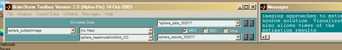
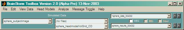
The BrainStorm (BST) Toolbar is always present in the upper lefthand corner of the desktop, with the Messages window just to its right:

BrainStorm Toolbar Operations

A quick New User guide to the more common functions:

File

Use the Data Manager to view and organize your data.

Use Quit to quit BrainStorm (but not Matlab).

Edit

Layout: Open the Layout Manager for adjusting where the BrainStorm desktop lies, and for managing the open BST windows.

Snap All: Set all of the open windows back into their proper positions.

View Data

Click this menu item to load the currently selected data into the Data Viewer manager. From that manager, data and results can be viewed in several different methods, and expert analyses can be executed on data.

Head Models

Default to generate a default volume grid of dipoles in parametric modeling.

Advanced to generate a variety of head models on a variety of grids.

Analyze

These items are designed to run scripts that perform the indicated analysis with a minimum of user input. For more expert interaction with these functions, see the menu item View Data and the pull-down menu for Analysis in the Data Viewer manager.

Message Toggle

Clicking on this item menu toggles the messages window between full screen and small size.

Help

Several levels of help, generally opening in the Matlab browser window. Please be patient the first time the Matlab Help Browser, since Matlab generally takes several seconds to create and load their internal browser.

Sample Default Session

Data Manager

Open the Data Manager and select the Default Database:

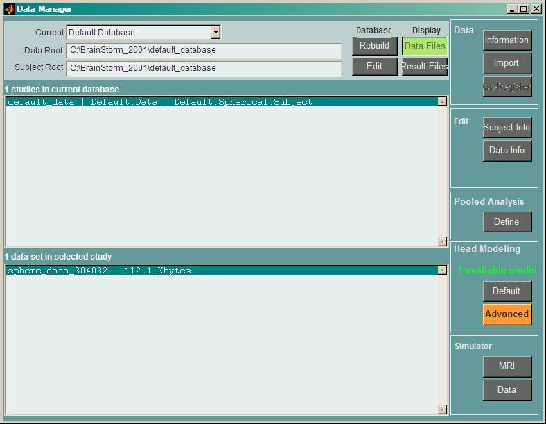
Click on the data set “sphere_data” (which may have a different hash extension than that shown above).

Execute Default Analysis

In the BST Toolbar under Analyze, click on RAP-MUSIC

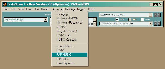
This toolbar will fully execute the analysis with minimal user input. The final result will be a pair of screens such as these:

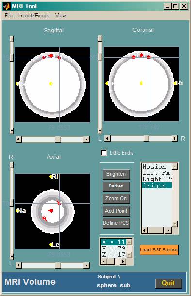
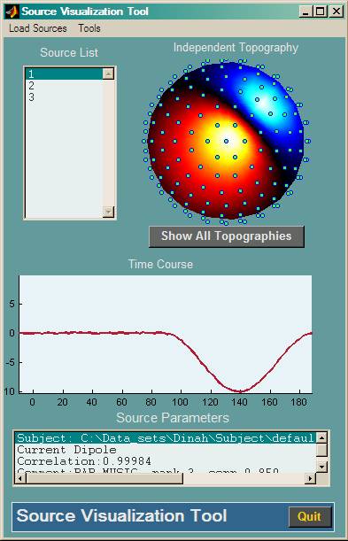
Click on each source number in succession in the right screen’s Source List to see each dipole individually in the MRI window on the left.

Expert Analysis

We now walk through the steps that were automatically executed above. First, let’s clean up the windows from the above analysis. In the BST toolbar, click on Edit -> Window Layout. In the Layout Window Manager, press Close All. In the Windows list under Toolbars, click on Parameters RAP-MUSIC to bring up that vertical toolbar, and close it.

Now click View Data in the BST Toolbar, which reloads the current data into the Data Viewer.

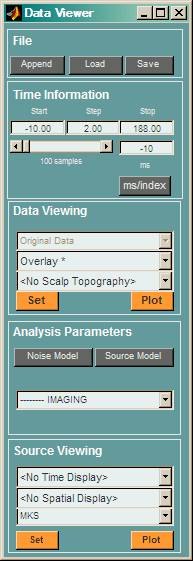
Under Data Viewing, press Plot.

In Analysis Parameters, pull down the popup menu to RAP-MUSIC and release. The Parametric Estimation Data Selector window opens,

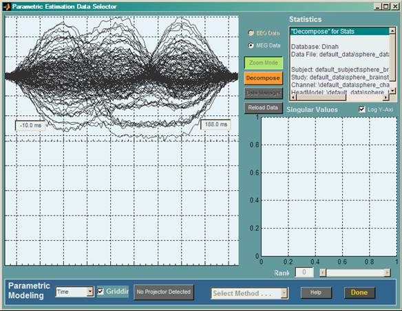
Press Decompose to decompose the data into its signal and noise subspace. A hypothesis test has automatically selected a putative rank. Adjust the rank as desired in the slider, observing the effects on the signal and noise subspace, with a tendency to overspecify the signal subspace rank. Rubber-band zoom on the singular values for a closer inspection. Press Done for the desired rank.

The RAP-MUSIC parameters toolbar opens:

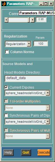
Select Regularization in the popup menu to be Tikhonov Condition 10, and press Execute. The resulting figures should be the same, assuming rank 3 or greater was chosen for the default data.

Further Data Investigation

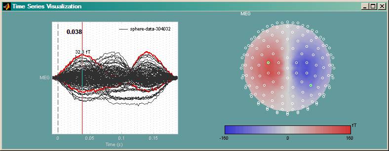
Under Data Viewing, pull down <No Scalp Topography> and select 3D Sphere.

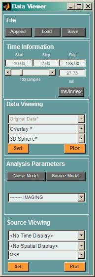
Press Plot to see an overlay plot of all channels and a corresponding spherical view of the fields at a sphere fit to the sensors. Grab and center the vertical red cursor to about 0.038 seconds. The spatial display shows the pattern at that time instance. Click on a sensor site to highlight the corresponding time waveform (toggled red) in the overlay plot, or click on a waveform to see the corresponding sensor site (toggled green).